Ellipse fitting algorithm

The ellipticity of the diffraction pattern is determined from an iso-intensity curve. A slight misalignment of the camera with respect to the orthogonal diffraction pattern is compensated for with the new tilted ellipse fit.

Ellipse fit.

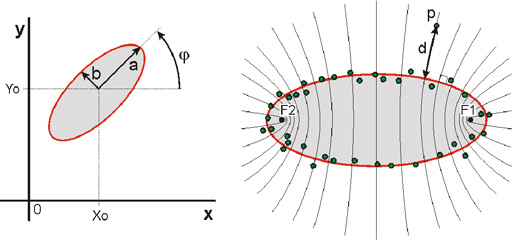
The orientation of the diffraction pattern in the video image depends on the orientation of the camera with respect to the measuring geometry. The diffraction pattern is therefore described by the equation of a tilted ellipse. (References 1 1. Ahn S.J., Rauh W., Geometric least squares fitting of circle and ellipse, Int. J. Pattern Recognit. Artif. Intell., vol. 13:(7), pp. 987-996, 1999., 33 Hart D., Rudman A.J., Least-squares fit of an ellipse to anisotropic polar data: Application to azimuthal resistivity surveys in karst regions, Computers & Geosciences, vol. 23:(2), pp. 189-194, 1997.) The ellipse parameters (see Figure 4 section a). namely location (x₀,y₀), orientation (j) and axes (A,B) are obtained by least squares fitting of the data points to the edge of the ellipse.(References 1 1. Ahn S.J., Rauh W., Geometric least squares fitting of circle and ellipse, Int. J. Pattern Recognit. Artif. Intell., vol. 13:(7), pp. 987-996, 1999., 33 Hart D., Rudman A.J., Least-squares fit of an ellipse to anisotropic polar data: Application to azimuthal resistivity surveys in karst regions, Computers & Geosciences, vol. 23:(2), pp. 189-194, 1997.)

Outlier rejection.

The ellipse parameters are heavily biased if outliers exist in the data points, or when part of a neighbouring cell coexists in the rectangular analysis region. The fitting algorithm is therefore encapsulated by an iterative procedure that skips the most-distant data point until all data points are within 10 pixels from the fit. The procedure rejects patterns if the remaining number of pixels drops below a specified number (50).

Distance to ellipse.

The distance of a data point to the obtained ellipse has to be calculated in order to reject outliers. Calculating this distance requires solving a quadratic equation, which is an inefficient procedure. A good approximation can be obtained using orthogonal hyperbola.(References 50 Rosin P.L., Ellipse fitting using orthogonal hyperbolae and Stirling's oval, Graphical Models and Image Processing, vol. 60:(3), pp. 209-213, May 1998., 51 Rosin P.L., Analysing error of fit functions for ellipses, Pattern Recognit. Lett., vol. 17, pp. 1461-1470, 1996.) Confocal ellipses and hyperbola intersect orthogonally (see Figure 4 section b). This property is exploited to find the confocal hyperbola that crosses a specific data point. The distance from the data point to the point of intersection between the ellipse and the hyperbola provides a good approximation of the shortest distance to the ellipse.(References 50 Rosin P.L., Ellipse fitting using orthogonal hyperbolae and Stirling's oval, Graphical Models and Image Processing, vol. 60:(3), pp. 209-213, May 1998., 51 Rosin P.L., Analysing error of fit functions for ellipses, Pattern Recognit. Lett., vol. 17, pp. 1461-1470, 1996.) The average distance of the edge pixels to the best-fit ellipse is defined as the Error Of Fit (Eof) parameter.

Accuracy of ellipse parameters.

The accuracy of the ellipse parameters is determined in one of two possible ways.

1. If one configures the software to analyze a certain number of diffraction patterns in order to reduce measurement inaccuracy, the programs displays the mean and standard deviation for each of the obtained ellipse parameters, and of the derived parameters (such as the EI).
2. If only one diffraction pattern is analyzed, which can be configured, e.g., for RBC-stability testing, parameter accuracy will be estimated using the Bootstrap method.(References 47 Press W.H., Teukolsky A.A., Vetterling W.T., Flannery B.P., Quick-and-dirty monte carlo: The bootstrap method, in: Numercal recipes in C, The art of scientific computing, Cambridge University Press, 2nd ed., pp. 691-694, 1992 (ISBN: 0-521-43108-5)., 60 Thomas G.E., Use of the bootstrap in robust estimation of location, The Statistician, vol. 49:(1), pp. 63-77, 2000.) This method takes M random data points from the set of N that remained after outlier rejection. M is normally taken equal to N resulting in a new hypothetical data set in which some data points appear more than once while others are omitted. By repeatedly (300x) generating these hypothetical data sets from the original set, and by fitting each set to the equation of a tilted ellipse, a distribution is obtained for each of the five ellipse parameters. The average value is a good estimate of the true parameter while the standard error serves to indicate the accuracy of the estimate.

Normally, the diffraction pattern is displayed on an orthogonal base and the orientation angle (j) will not be of value in ektacytometry. Therefore A is taken the axis closest to the vertical and B is taken the axis closest to the horizontal. With this definition EI can be negative when the diffraction pattern is rotated over 90º, which happens when the cells orient differently in shear flow, e.g., in sickle cell anemia (Reference 9 Bessis M., Mohandas, N., Feo C., Automated ektacytometry: A new method of measuring red cell deformability and red cell indices, Blood cells, vol. 6, pp. 315-327, 1980.) or elliptocytosis.(References 18 Dobbe J.G.G., Hardeman M.R., Streekstra G.J., Strackee J., Ince C., Grimbergen C.A., Analyzing red blood-cell deformability distributions, Blood Cells, Molecules, and Diseases, vol. 28:(3), pp. 373-384, May/Jun 2002., 15 Dobbe J.G.G., Engineering developments in hemorheology, PhD Thesis, University of Amsterdam, Sept. 2002.)

Note that the accuracy of the fit also depends on the number of edge coordinates that are extracted from the image. The number of edge coordinates can be increased by fitting more than one intensity level, at the cost of computational speed.